RHEED Image Stacks

This notebook demonstrates how to load and process a sequence of RHEED images acquired during molecular beam epitaxy (MBE).

import matplotlib.pyplot as plt
import numpy as np
from pathlib import Path

import xrheed

🎉 xrheed v2.1.0 loaded!

Loading a Series of RHEED Images

In this example, we work with a sequence of BMP images located in the deposition directory. To load the data, we first need to prepare the following:

• A list of file paths (preferably as pathlib.Path objects)

• A name for the stack dimension

• A list or vector of precise coverage values corresponding to each image in the sequence

Note: The allowed stack dimension options are defined in constants.CANONICAL_STACK_DIMS.

Valid values include: alpha, beta, coverage, time, temperature, current.

image_dir = Path("example_data/deposition")

# Get all BMP files and sort them numerically by the number in the filename
image_paths = sorted(
    image_dir.glob("*.BMP"),
    key=lambda p: int(p.stem.split("_")[-1])
)

# Typically the list of paths could be generated in a simpler way:
# image_paths = list(image_dir.glob("*.BMP"))

n_stack = len(image_paths)

stack_dim = 'coverage'
deposition_rate = 2.54 # Hz per image

stack_coordinate = np.linspace(0.0, n_stack * deposition_rate, n_stack)

The data can be loaded using the same xrheed.load_data() function by providing a list of paths instead of a single path. In addition, the stack_dim and stack_coords parameters must be specified.

To correctly interpret the data format, the plugin argument must also be provided. This should point to a specific plugin capable of handling the structure and metadata of the dataset being loaded.

As clearly visible those images show significant shift in y direction, that is why we first apply the manual shift and later use automatic adjustment.

Next, we manually set the center of each image using the set_center_manual() function. If numeric values for center_x and center_y are provided, the same shift is applied uniformly to all images in the stack.
Optionally, if a list or vector of center_x values is provided (with length equal to the number of images), each image will be shifted according to its corresponding value.

rheed_data = xrheed.load_data(
    image_paths,
    plugin="dsnp_arpes_bmp",
    stack_dim=stack_dim,
    stack_coords=stack_coordinate,
)

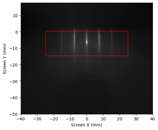
rheed_data.ri.screen_roi_width = 40
rheed_data.ri.screen_roi_height = 50

# Plot the image to inspect the alignment
rheed_data.ri.plot_image(auto_levels=1.0)

center_x = -1.0
center_y = -8.0
plt.plot(center_x, center_y, '+')

plt.show()

# Set approximate center of the images
rheed_data.ri.set_center_manual(center_x, center_y)

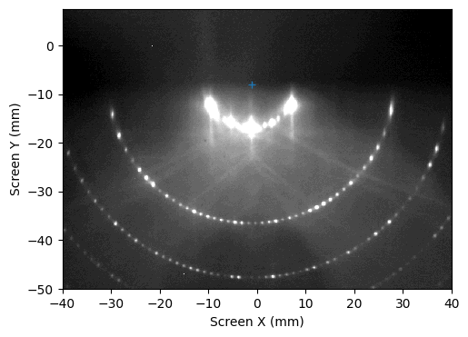
rheed_data.ri.set_center_auto()

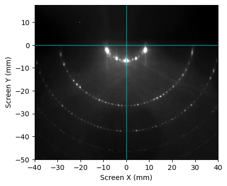
Plot the Images from the Stack

The plot_image() function displays the first image from the stack by default. Alternatively, a specific image can be shown by providing the stack_index keyword argument.

If stack_index is set, the corresponding image at that index in the stack will be plotted instead of the default first image.

rheed_data.ri.plot_image(
    show_center_lines=True,
    auto_levels=0.2,
    stack_index=0,
)
plt.show()

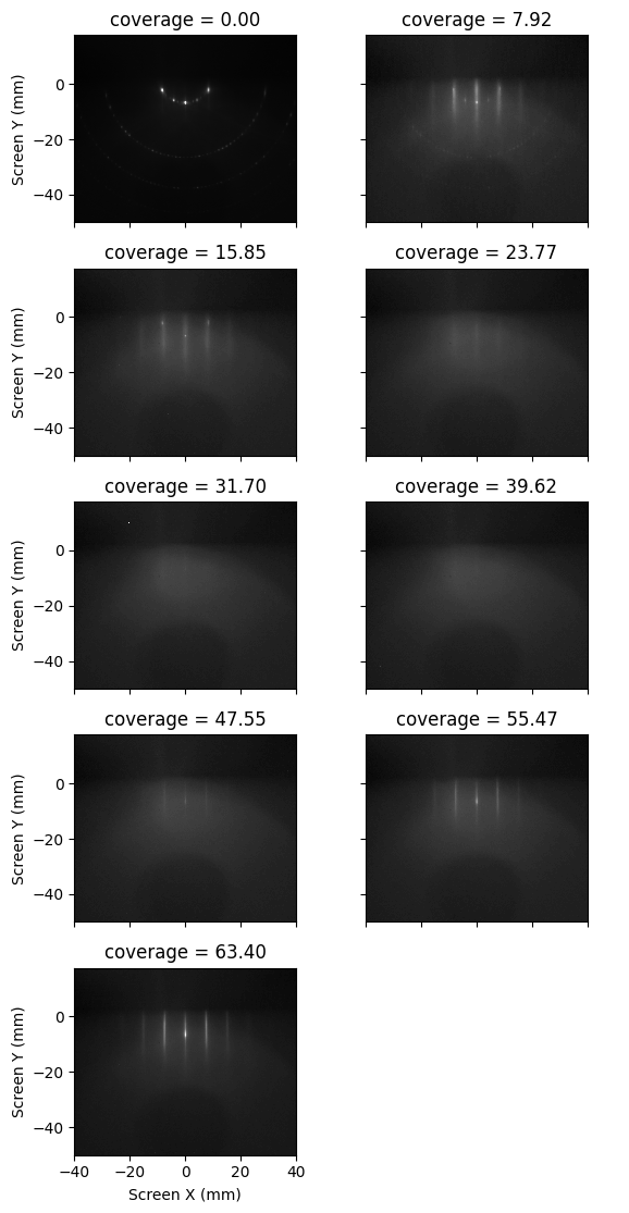
The plot_images() function from the plotting module can be used to display all images in the stack.

To visualize a subset of the images, standard xarray slicing can be applied. For example, to show every third image in the stack, use slicing as demonstrated below.

from xrheed.plotting import plot_images

plot_images(rheed_data.isel(coverage=slice(None, None, 3)), ncols=2)
plt.show()

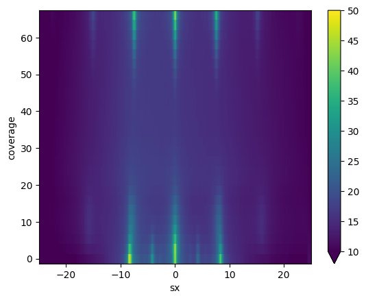
RHEED Stack Profiles

The get_profile method, available through the ri accessor, returns a 2D dataset extracted from a 3D RHEED stack. By default, it integrates the data along the screen’s Y direction, similar to how profiles are obtained from a single RHEED image.

Note: If show_origin is set to True, it is also possible to pass the stack_index argument to visualize the origin area. In this case, the origin will be marked by a rectangle on the selected image from the stack, rather than on the default first image.

profile_2d = rheed_data.ri.get_profile(
    center=(0, -7), 
    width=50, 
    height=15, 
    show_origin=True, 
    stack_index=25
)

Plotting a 2D Profile

The returned profile is an xarray.DataArray and can be visualized using its built-in .plot() method, as shown below.

profile_2d.plot(vmin=10, vmax=50)
plt.show()

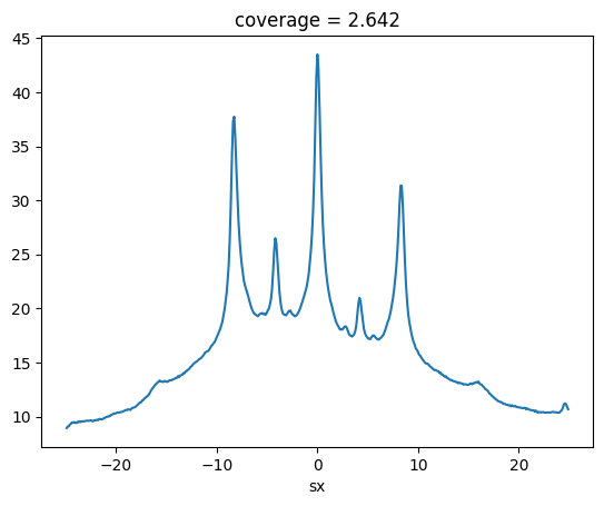
Extracting a Single Profile

Optionally, it is possible to extract a single profile from a 2D stack using standard slicing or selection operations. This allows for flexible access to specific regions or lines within the dataset without invoking the full get_profile method.

profile_2d.isel(coverage=1).plot()
plt.show()

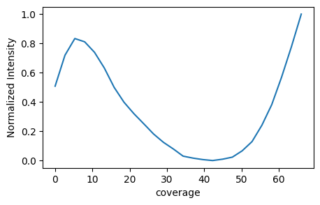
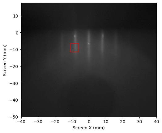
1D Profile from a 3D Stack

The default behavior of the get_profile method can be modified by providing the reduce_over keyword argument. Allowed options are: "sy", "sx", and "both".

If the "both" option is selected, the profile is integrated over the entire selection area. This is particularly useful for spot analysis during MBE growth, for example, to record RHEED oscillations.

profile_1d = rheed_data.ri.get_profile(
    center=(-8.5, -9),
    width=5,
    height=5,
    reduce_over="both",
    show_origin=True,
    stack_index=5,
)

Finally, the profile, returned as an xarray.DataArray, can be plotted using its internal .plot() method. Alternatively, it can be visualized using the plot_profile() method available via the rp accessor.

profile_1d.rp.plot_profile()
plt.show()