Spot Calculation Using Ewald Construction

This notebook demonstrates how to use the xrheed.kinematics module to superimpose calculated diffraction spot positions onto a RHEED image.

Before proceeding, it is recommended to review the Geometry and Kinematic Diffraction Model sections of the documentation for a foundational understanding of the underlying principles.

import matplotlib.pyplot as plt
from pathlib import Path

import xrheed

🎉 xrheed v2.1.0 loaded!

Preparation of RHEED Image Data

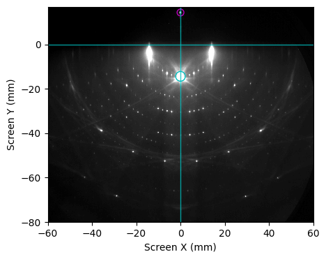
As a representative example, we utilize a reflection high-energy electron diffraction (RHEED) image acquired from a clean Si(111) surface exhibiting the characteristic (7×7) surface reconstruction.

The incident electron beam was aligned along the crystallographic direction \([11\bar{2}]\). Consequently, the horizontal axis of the RHEED image corresponds to the \([1\bar{1}0]\) direction.

image_dir = Path("example_data")
image_path = image_dir / "Si_111_7x7_112_phi_00.raw"

rheed_image = xrheed.load_data(image_path, plugin="dsnp_arpes_raw")

# Align the image rotation
rheed_image.ri.rotate(-0.4)

# Set the screen ROI
rheed_image.ri.screen_roi_width = 60
rheed_image.ri.screen_roi_height = 80

# Apply automatic center search and calculate the incident angle
rheed_image.ri.set_center_auto(update_incident_angle=True)

# Use automatic levels adjustment
rheed_image.ri.plot_image(
    auto_levels=0.5, show_center_lines=True, show_specular_spot=True
)

plt.show()

Construction of the 2D Lattice Object

To begin, we calculate the positions of the (1×1) diffraction spots using a hexagonal two-dimensional lattice with a lattice constant of 3.84 Å.

The lattice can be instantiated using the Lattice class, which accepts real-space basis vectors.

Additional methods available for lattice generation include:

• from_bulk_cubic: Constructs the lattice from a bulk cubic crystal by specifying the lattice constant a, the cubic_type, and the crystallographic plane (currently limited to low-index planes).

• from_surface_hex: Generates a two-dimensional hexagonal lattice by specifying only the surface lattice constant.

All available options are demonstrated below to generate the same lattice.

from xrheed.kinematics import Lattice

# Manually define a 2D lattice using real-space basis vectors.
# This example uses a hexagonal configuration with a lattice constant of 3.84 Å.
lattice = Lattice([0.0, 3.84], [3.325, 3.84 * 0.5], label="manual generation")
print(lattice)

# Generate a surface lattice derived from a bulk cubic crystal.
# Specify the lattice constant, crystal type (FCC), and Miller plane (111).
lattice = Lattice.from_bulk_cubic(
    a=5.43, cubic_type="FCC", plane="111", label="from bulk"
)
print(lattice)

# Create a 2D hexagonal lattice using a simplified method.
# Only the surface lattice constant is required.
lattice = Lattice.from_surface_hex(a=3.84, label="as hex lattice")
print(lattice)

Lattice: manual generation
a1 = [0.000, 3.840] A
a2 = [3.325, 1.920] A
Lattice: from bulk
a1 = [0.000, 3.840] A
a2 = [3.325, 1.920] A
Lattice: as hex lattice
a1 = [0.000, 3.840] A
a2 = [3.326, 1.920] A

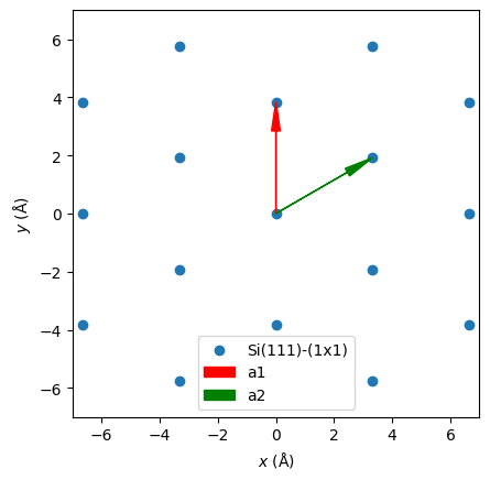
Generation and Visualization of the (1×1) Surface Lattice

Finally, we generate a (1×1) surface lattice using a lattice constant of 3.84 Å, and visualize it using the plot_real method.

The space_size parameter defines the plotting boundaries in the x and y directions, which correspond to the in-plane coordinates of the sample surface.

si_111_1x1 = Lattice.from_surface_hex(a=3.84, label="Si(111)-(1x1)")

si_111_1x1.plot_real(space_size=7.0, show_vectors=True)
plt.legend()
plt.show()

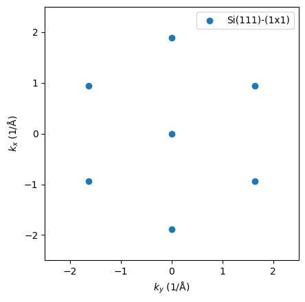
Reciprocal Lattice Visualization

The reciprocal lattice is generated automatically and can be visualized using the appropriate plotting method.

Note: In the reciprocal space plot, the vertical (y) axis represents the \(k_x\) component, which corresponds to the direction of the incident electron beam.

si_111_1x1.plot_reciprocal(space_size=2.5)
plt.legend()
plt.show()

Lattice azimuthal orientation

By default, the hexagonal lattice is constructed such that the x axis - approximately aligned with the electron beam direction-corresponds to the crystallographic \([11\bar{2}]\) direction.

If the sample orientation differs, the lattice can be rotated accordingly. This can be achieved either manually or by specifying the alpha angle extracted from the RHEED image. In the latter case, the rotation is applied within the Ewald class object.

Upon rotation, both the real-space and reciprocal-space representations are updated automatically to reflect the new orientation.

The Ewald Class

With the two essential components prepared:

• rheed_image: a loaded and properly aligned RHEED image,

• si_111_1x1: a defined surface lattice object,

the diffraction spot positions can be computed using kinematic theory based on the Ewald construction. The Ewald object is initialized using these two inputs.

Although the RHEED image is technically optional, it is strongly recommended for realistic simulations. It provides key experimental parameters such as:

• the sample-to-screen distance,

• screen scaling factors,

• and the incident angle \(\beta\) of the electron beam.

Note: The Ewald object internally generates its own lattice instance, which can be independently scaled or rotated to achieve precise alignment with experimental data.

from xrheed.kinematics import Ewald

ew_si_111 = Ewald(lattice=si_111_1x1, image=rheed_image)

print(ew_si_111)

Ewald Class Object: Si(111)-(1x1)
  Ewald Radius            : 71.36 1/Å
  Image azimuthal angle:  : 0.00°
  Incident angle          : 2.66°
  Real Lattice Scale      : 1.00
  Screen Scale            : 9.31 px/mm
  Sample-Screen Distance  : 309.2 mm
  Screen Shift X          : 0.00 mm
  Screen Shift Y          : 0.00 mm
  Reciprocal Vector b1    : [0.94, -1.64] 1/Å
  Reciprocal Vector b2    : [-1.89, 0.00] 1/Å

Once the Ewald object is initialized, diffraction spot positions are automatically calculated.

The plot method displays the computed spots, optionally superimposed on the RHEED image - if available and if the show_image argument is set to True.

fig, ax = plt.subplots(figsize=(5, 4))

ew_si_111.plot(ax=ax, show_image=True, show_center_lines=True, auto_levels=1.0)
plt.show()

Fine Adjustment

Typically, the incident angle may not be perfectly set, and the image scaling may also require refinement. Two methods are available for adjusting the calculated spot positions:

Adjusting the Ewald Object

For temporary corrections or simpler analyses, it is recommended to directly modify the following attributes of the Ewald object:

• incident_angle

• shift_x

• shift_y

• fine_scaling

These adjustments are stored independently of the original RHEEDImage object.

Adjusting the RHEEDImage Object

If more fundamental parameters-such as screen_scale-need to be corrected, these changes should be applied directly to the RHEEDImage object. In such cases, the Ewald object must be re-created to reflect the updated image parameters.

The same applies to x/y shifts of the RHEED image, as described in the Getting Started notebook.

Fine Adjustment Example

Below, we apply corrections directly to the Ewald object and visualize the results using the plot method.

This approach allows for quick tuning of parameters such as the incident angle and screen alignment, without modifying the original RHEEDImage object.

shift_y = -0.1
fine_scaling = 1.0

ew_si_111.shift_y = shift_y
ew_si_111.fine_scaling = fine_scaling

ew_si_111.plot(auto_levels=1.0, marker="d", s=30, alpha=0.3, color="c")
plt.show()

Adding the reconstruction

Having the (1x1) structure well adjusted we can add the (7x7) reconstruction.

si_111_7x7 = Lattice.from_surface_hex(a=3.84 * 7, label="Si(111)-(7x7)")
si_111_7x7

Lattice: Si(111)-(7x7)
a1 = [0.000, 26.880] A
a2 = [23.279, 13.440] A

Create Ewald object for new lattice, and optionally copy already adjusted attributes.

ew_si_111_7x7 = Ewald(si_111_7x7, rheed_image)

ew_si_111_7x7.shift_y = shift_y

ew_si_111_7x7.plot(auto_levels=1.0)
plt.show()

Final Image

Finally, a plot is prepared and saved, showcasing both reconstructions.

For improved clarity, a high-pass filtered image is used in this visualization.

from xrheed.preparation.filters import high_pass_filter

sigma = 5.0  # in mm
sigma_px = sigma * rheed_image.ri.screen_scale
threshold = 0.8

hp_rheed_image = high_pass_filter(rheed_image, sigma=sigma, threshold=threshold)

fig, ax = plt.subplots(figsize=(5, 4), constrained_layout=True)

hp_rheed_image.ri.plot_image(ax=ax, vmin=7, vmax=30)

ew_si_111_7x7.plot(
    ax=ax, show_image=False, marker=".", s=5, alpha=0.5, color="y"
)

ew_si_111.plot(ax=ax, show_image=False, marker="d", s=40, alpha=0.5, color="c")

ax.set_xlabel(" ")
ax.set_ylabel(" ")
ax.set_xticks([])
ax.set_yticks([])
ax.set_ylim(-80, 5)
fig.set_dpi(100)
plt.show()
# fig.savefig()