Ewald Spot Matching

This notebook demonstrates the use of the Ewald class methods from the kinematics module to determine either the surface reconstruction orientation or the lattice constant.

We assume that the surface exhibits a well-defined and visible (1×1) structure, which may be used for image scaling. Alternatively, the image may be calibrated and aligned using external reference data.

Next, we construct a lattice object representing, for example, a two-dimensional hexagonal lattice with unknown azimuthal orientation and lattice constant. This scenario is typical for complex surface reconstructions such as (√7 × √7) R19.1°, which often produce intricate RHEED (Reflection High-Energy Electron Diffraction) patterns.

Another common situation arises when the RHEED image is acquired along a non-symmetric crystallographic direction, often due to experimental constraints (e.g., lack of azimuthal rotation). In such cases, the diffraction pattern may be difficult to interpret, complicating the analysis of surface reconstruction.

Currently, the supported functionality includes the following scenarios:

• (I) Determination of the azimuthal orientation of a predefined lattice (hexagonal or rectangular) with fixed lattice vectors — match_alpha() method.

• (II) Scaling analysis of a hexagonal or rectangular lattice with a fixed azimuthal orientation — match_scale() method.

• (III) Simultaneous determination of both scaling and azimuthal orientation for hexagonal or rectangular lattices, assuming a fixed ratio between lattice vectors — match_alpha_scale() method.

Algorithm Explained

The core idea of the algorithm implemented here is as follows:

1. Define the lattice structure expected to occur on the sample surface.

2. Overlay the lattice onto the experimental RHEED image.

3. Generate a mask composed of elliptical spots, positioned according to the calculated diffraction spot locations derived from Ewald sphere construction.

4. Integrate the pixel intensities within the masked regions to compute a single scalar value—referred to as the matching_coefficient. This coefficient quantifies the agreement between the expected lattice and the experimental RHEED pattern. A higher value indicates better correspondence.

5. Systematically rotate or scale the lattice and repeat the above steps to evaluate the matching_coefficient across different configurations.

By scanning over a range of possible scaling factors and orientations, the configuration yielding the highest matching_coefficient serves as a strong candidate for the actual lattice present on the sample.

Cache Data

The calculations shown below can be time-consuming. In a 2D case, scanning a wide range of scaling factors and azimuthal angles with small step sizes may take several hours on an average computer to generate a complete matching map.

To optimize performance, the results are automatically serialized using dill and stored in the cache directory. Only one .dill file is saved per call to a specific match_* method. When these methods are invoked, they first check for an existing cache file.

To force recalculation, either delete the corresponding cache file or set Ewald.use_cache = False for the specific Ewald object.

import matplotlib.pyplot as plt
import numpy as np
from pathlib import Path

import xrheed
from xrheed.preparation.filters import high_pass_filter

🎉 xrheed v2.1.0 loaded!

Prepare the RHEED Data

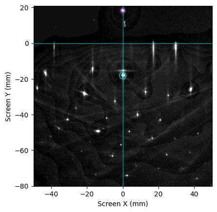
In this example, we use a RHEED image obtained from a Si(111) with Ag induced (√3 × √3) R30° surface reconstruction, where the sample is azimuthally misoriented by approximately 15°.

The goal is to determine both the lattice constant and the azimuthal orientation relative to the incident electron beam.

For this analysis, we define a region of interest (ROI) that excludes the central portion of the image, focusing instead on peripheral diffraction features.

image_dir = Path("example_data")
image_path = image_dir / "Si_111_r3Ag_thB_phi15.raw"

rheed_image = xrheed.load_data(image_path, plugin="dsnp_arpes_raw")

# Rotate the image
rheed_image.ri.rotate(-0.2)

# Fine adjustment of the image center
shift_x = -4.4
shift_y = -4.2
rheed_image.ri.set_center_manual(center_x=shift_x, center_y=shift_y)

# Set the incident angle
rheed_image.ri.incident_angle = 3.35

# Set the azimuthal angle to 0 (default) although it is definitely non zero here
rheed_image.ri.azimuthal_angle = 0.0

# Setup the screen roi
rheed_image.ri.screen_roi_width = 50
rheed_image.ri.screen_roi_height = 80

# use high pass filter to reduce inelastic scattering features
rheed_image = high_pass_filter(rheed_image, sigma=3.0, threshold=0.8)

# Prepare the plot
fig, ax = plt.subplots()

# Use automatic levels adjustment and show specular spot
rheed_image.ri.plot_image(ax=ax, auto_levels=0.2, show_specular_spot=True, show_center_lines=True)

plt.show()

Scenario I: Unknown Azimuthal Orientation of the Sample

First, we present the simplest case: the expected surface structure (type and lattice constant) is known, but the azimuthal orientation of the sample is unknown.

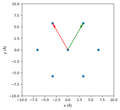
Create the Expected Lattice

We define the expected lattice as Si(111)-(√3 × √3) R30° in this example.

from xrheed.kinematics import Lattice

expected_lattice = Lattice.from_surface_hex(a=3.84 * np.sqrt(3.0), label="r3-Ag")
expected_lattice.rotate(30.0)

expected_lattice.plot_real()
plt.show()

Create an Ewald Object

Next, we create an instance of the Ewald class using the expected lattice and the experimental RHEED image.

In this example, the α angle is set to its default value of 0°, which is acceptable for demonstration purposes, although it does not reflect the actual experimental geometry. As a result, the calculated diffraction spots will not align precisely with those observed in the RHEED image.

from xrheed.kinematics import Ewald

ew = Ewald(expected_lattice, rheed_image)
ew.ewald_azimuthal_rotation = 15.0
ew.plot(auto_levels=0.2)
plt.show()

Test Plot

A convenient starting point is to generate a test plot that overlays calculated Ewald diffraction spots onto a RHEED image in order to explore possible azimuthal orientations.

The Ewald class uses the azimuthal angle stored in the RHEED image metadata as a fixed experimental reference. To test or fine-tune the orientation of the theoretical Ewald construction, a relative rotation can be applied using the ewald_azimuthal_rotation attribute.

By manually adjusting this value, the user can interactively rotate the Ewald construction with respect to the image while keeping the experimental azimuth unchanged.

fig, ax = plt.subplots()
cmap = plt.get_cmap("hot")

# Plot the RHEED image
rheed_image.ri.plot_image(ax=ax, auto_levels=0.2)

# Check the rotation range
alpha_vector = np.arange(10.0, 20.0, 1.0)

# Loop over alpha values and plot
for i, alpha in enumerate(alpha_vector):
    # Set the azimuthal rotation
    ew.ewald_azimuthal_rotation = alpha

    # normalize i into [0,1] for colormap
    color = cmap(i / (len(alpha_vector) - 1))
    ew.plot(ax=ax, show_image=False, edgecolor=color, facecolor="none", 
            marker="o", linewidth=0.8, s=20)

plt.show()

Spot Probe

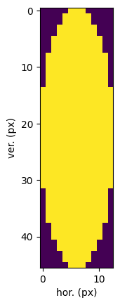
Each spot is generated with an elliptical shape, defined by its width and height (in mm). The default dimensions are specified as constants within the Ewald class.

In general, the spot size should be chosen to match the actual shape of the diffraction spots observed in the RHEED image.

The following guidelines apply:

• Larger probing spot size: increases computation time, reduces sensitivity, but performs better when scanning over coarse steps (e.g., ~1° in azimuthal orientation).

• Smaller probing spot size: decreases computation time and increases sensitivity, but may fail to detect the correct orientation when using coarse angular steps.

To manually set the spot dimensions, use the method set_spot_size(width, height), where both parameters are specified in millimeters.

# Set the spot size
ew.set_spot_size(1.5, 5.0)

# Show the spot structure
plt.imshow(ew.spot_structure)
plt.xlabel("hor. (px)")
plt.ylabel("ver. (px)")
plt.show()

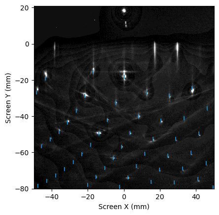
How It Works

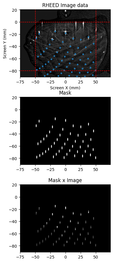
To better understand the process, the figure below illustrates three components:

• Top: The RHEED image overlaid with calculated spot positions (temporarily using the correct azimuthal alignment).

• Center: A binary True/False mask used to evaluate the match between expected and observed diffraction spots.

• Bottom: The RHEED image multiplied by the mask, highlighting only the regions considered in the matching calculation.

This visualization is useful for validating the spot shape configuration and ensuring that the mask accurately captures the relevant diffraction features.

fix, axs = plt.subplots(3, 1, figsize=(4, 11))

# Use a close to real azimuthal orientation to rotate the Ewald class
ew.ewald_azimuthal_rotation = 15.0

ax = axs[0]
ew.plot(ax=ax, show_roi=True, auto_levels=0.4, marker=".")
ax.set_title("RHEED Image data")

ax = axs[1]
ew.plot_spots(ax=ax)
ax.set_title("Mask")

ax = axs[2]
ew.plot_spots(ax=ax, show_image=True, vmin=0, vmax=15)
ax.set_title("Mask x Image")

plt.show()

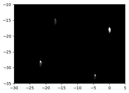
Adjusting the Spot Size

To fine-tune the spot size, the plot_spots method can be used with the parameter show_image=True. In this mode, the product of the binary mask and the RHEED image is displayed, allowing visual inspection of how well the spot structure aligns with the actual diffraction features.

For detailed examination, it is recommended to zoom in using narrow x and y axis limits. This helps verify whether the elliptical spot shape accurately matches the RHEED spots.

ew.ewald_azimuthal_rotation = 15.0

spot_width_mm = 0.8
spot_height_mm = 2.0

ew.set_spot_size(spot_width_mm, spot_height_mm)

fix, ax = plt.subplots(figsize=(5, 4))

ew.plot_spots(ax=ax, show_image=True, vmin=0, vmax=80)

ax.set_xlim(-30, 5)
ax.set_ylim(-35, -10)

plt.show()

Final Step: Check the Reconstruction Orientation

In the final step, we evaluate all possible azimuthal orientations. For a hexagonal lattice, this typically spans from −30° to +30°, due to its inherent threefold rotational symmetry.

We begin by creating an alpha_vector that defines the range of azimuthal angles to test. Then, we call the appropriate method to compute the matching coefficient for each orientation.

At this stage, it is advisable to use a relatively large spot size. This reduces sensitivity but allows for robust matching across a broader angular range. Once a candidate orientation is identified, the spot size can be reduced to refine the result with higher precision.

alpha_vector = np.arange(-30, 30.0, 0.5)
match_vector = ew.match_alpha(alpha_vector)

Loading cached result from cache/cache_match_alpha.dill

fig, ax = plt.subplots(figsize=(5, 4))

match_vector.plot(ax=ax)

ax.set_xlabel("Azimuthal rotation (alpha)")
ax.set_ylabel("Matching coef. (a. u.)")

alpha_max = match_vector.idxmax(dim="alpha").item()
print(f"Maximum match at scale factor = {alpha_max:.3f}")

plt.show()

Maximum match at scale factor = 15.000

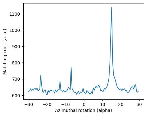
Results Interpretation

As expected, there is a distinct peak around α = 15°, which corresponds to the intentional azimuthal rotation applied during acquisition of this RHEED image.

To refine the orientation estimate, we reduce the spot size and narrow the α range around this angle. Additionally, we decrease the angular step to, for example, 0.1°. These adjustments improve sensitivity and allow for more precise matching by better aligning the mask with the actual diffraction spot geometry.

Scenario II: Unknown Lattice Constant

In this scenario, we assume that the azimuthal orientation of the sample is known, but the lattice constant is unknown.

To determine the correct lattice constant, we use the match_scale method of the Ewald class, as shown below.

Note: the scale refers to real-space dimensions. For example, a scale factor of 2 corresponds to a (2×2) surface superstructure.

Prepare Expected Lattice

First, we create an Ewald object using a lattice with an approximate lattice constant—ideally close to the expected value. In this case, we use the (√3 × √3) R30° lattice as the initial structure.

# Expected lattice
expected_lattice = Lattice.from_surface_hex(a=3.84 * np.sqrt(3), label="r3-Ag")
expected_lattice.rotate(30.0)

# Create Ewald object
ew = Ewald(expected_lattice, rheed_image)

# Set the azimuthal orientation that is known in this scenario
ew.ewald_azimuthal_rotation = 15.0

We prepare the scale_vector centered around 1.0 to explore possible superstructures and identify the best match.

By scanning over a fine range of scale factors, we can pinpoint the configuration that yields the highest matching coefficient, indicating the most likely real-space lattice constant.

# Scale vector used for lattice scaling
scale_vector = np.arange(0.8, 1.3, 0.01)
match_vector = ew.match_scale(scale_vector)

Loading cached result from cache/cache_match_scale.dill

Plot the Results

fig, ax = plt.subplots(figsize=(5, 4))

match_vector.plot(ax=ax)

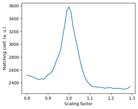
ax.set_xlabel('Scaling factor')
ax.set_ylabel('Matching coef. (a. u.)')

scale_max = match_vector.idxmax(dim="scale").item()
print(f"Maximum match at scale factor = {scale_max:.3f}")

plt.show()

Maximum match at scale factor = 1.000

Results interpretation

The peak in the plot indicates the best match occurring around a scaling factor of 1.0, which is consistent with expectations. This suggests that the initial lattice constant used in the Ewald object closely approximates the true surface structure.

Such a result confirms that no significant reconstruction or strain-induced distortion is present, and the observed RHEED pattern corresponds well to the assumed lattice geometry.

Scenario III: Unknown Scale and Azimuthal Orientation

In the third scenario, we aim to determine both the lattice scaling factor and the azimuthal orientation, which are initially unknown.

This combined search is particularly useful when analyzing complex surface reconstructions or when no prior calibration data is available.

Note I: The matching_coefficient is normalized by the number of diffraction spots. Since the number of spots changes discretely (in integer steps), this may introduce step-like artifacts in the results. To disable normalization and obtain raw matching values, set normalize=False when calling the matching method.

Note II: In this 2D case, in addition to normalization, there is another argument—flatten (enabled by default). This option subtracts a second-order polynomial fitted to the data, averaged along the α (azimuthal) direction. This correction compensates for nonuniform background intensity, which tends to decay at larger scaling factors as more diffraction spots fall within the region of interest (ROI).

Prepare Expected Lattice

In this case, we assume that the expected lattice corresponds to a surface reconstruction derived from the Si(111)-(1×1) structure.

By defining a lattice object that approximates this reconstructed geometry, we can proceed with a simultaneous scan over both azimuthal orientation and lattice scaling to identify the best match with the experimental RHEED image.

# Expected lattice Si(1x1)-(1x1) or some reconstruction of it
expected_lattice = Lattice.from_surface_hex(a=3.84, label="Si(111)-(1x1)")

ew = Ewald(expected_lattice, rheed_image)

# Scale vector used for lattice scaling
scale_vector = np.arange(0.8, 2.5, 0.025)
alpha_vector = np.arange(-30, 30, 0.5)

Calculate the Matching Map

Now we are ready to calculate the full matching map. This process involves scanning across a range of azimuthal orientations and scaling factors to identify the configuration that best matches the experimental RHEED pattern.

Note: This computation can be intensive and may take several hours depending on the resolution of the scan and the available computational resources.

To optimize performance, consider adjusting step sizes, or limiting the scan range during initial exploration. Once a promising region is identified, a refined scan can be performed for higher precision.

match_map = ew.match_alpha_scale(alpha_vector, scale_vector)

Loading cached result from cache/cache_match_alpha_scale.dill

Plot the Results

Below, we present the matching map generated from the combined scan over azimuthal orientation and lattice scaling. Several key points are marked on the plot and will be discussed in detail later.

This visualization helps identify regions of high matching coefficient, guiding the selection of optimal reconstruction parameters. Peaks in the map correspond to configurations where the simulated diffraction pattern closely aligns with the experimental RHEED image.

fig, ax = plt.subplots(figsize=(5, 4))

match_map.plot(ax=ax, vmin=100, vmax=1500, add_colorbar=False)

ax.set_ylabel('Azimuthal rotation (alpha)')
ax.set_xlabel('Scaling factor')

rec_A_scale = 1.0
rec_A_alpha = 14.9

ax.scatter(rec_A_scale, rec_A_alpha, marker=".", color="r", s=30)

rec_B_scale = 1.73
rec_B_alpha = -15.1

ax.scatter(rec_B_scale, rec_B_alpha, marker=".", color="m", s=30)

plt.show()

Interpreting the Results

The key features of interest in the matching map are located at the following coordinates:

• Scale = 1.0, α = +15° — Corresponds to the Si(111)-(1×1) lattice.

• Scale ≈ 1.7, α = −15° — Matches the (√3 × √3) R30° surface reconstruction.

Note: The matching map contains several sharp features, some of which are artifacts caused by occasional overlap between calculated spot positions and intense regions in the RHEED image. These artifacts can produce misleading peaks and should be interpreted with caution.

Additionally, there is a broader and less intense peak at Scale = 2.0, α = +15°. This feature originates from a (1×1) lattice scaled by a factor of 2, where every second calculated spot coincidentally aligns with bright regions in the experimental image.

While this produces a noticeable peak in the matching coefficient, it likely reflects an algorithm artifact rather than a true physical reconstruction.

Such cases underscore the importance of combining matching analysis with physical intuition and known surface symmetries.

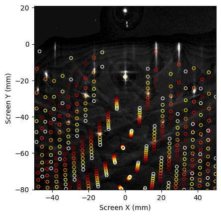
Summary

This analysis successfully identifies both the Si(111)-(1×1) structure and the Si(111)-(√3 × √3) R30° surface reconstruction. The matching map reveals distinct peaks corresponding to these configurations, confirming their presence in the experimental RHEED image.

Additionally, the sample appears to be rotated by approximately +15° relative to the high-symmetry [11-2] crystallographic direction, consistent with the observed azimuthal offset.

To visually confirm these findings, we now plot the two reconstructed lattices over the RHEED image using their respective rotation angles. This final step provides a direct comparison between calculated spot positions and experimental diffraction features, validating the accuracy of the matching procedure.

# Prepare the plot
fig, ax = plt.subplots(figsize=(5, 5))

rheed_image.ri.plot_image(
    ax=ax, show_specular_spot=False, show_center_lines=False, auto_levels=0.2
)

# Prepare and plot the first: (1x1) R+15 lattice
ew.ewald_azimuthal_rotation = rec_A_alpha
ew.lattice_scale = rec_A_scale
ew.ewald_roi = 20
ew.plot(ax=ax, show_image=False, color="r", marker=".")

# Prepare and plot the second lattice
ew.ewald_azimuthal_rotation = rec_B_alpha
ew.lattice_scale = rec_B_scale
ew.ewald_roi = 20
ew.plot(ax=ax, show_image=False, edgecolor="m", facecolor="none", marker="o", s=80)

plt.show()

Finally, it should be noted that the alignment between the calculated diffraction points and the experimental RHEED spots is not entirely perfect, indicating that the image was not precisely aligned in the data preparation steps.

Nonetheless, the matching was sufficiently accurate to resolve the key structural features and successfully interpret the surface reconstruction in this case.