Multi-Image Transformation
This example notebook demonstrates how to load and transform a series of RHEED images taken during sequential azimuthal rotations.
The rotation starts at \(\alpha = 0^\circ\), where the electron beam is aligned along the \([11\bar{2}]\) direction, and ends at \(\alpha = 30^\circ\), corresponding to alignment along the \([1\bar{1}0]\) direction.
import matplotlib.pyplot as plt
import numpy as np
from pathlib import Path
import xarray as xr

import xrheed
from xrheed.plotting.overview import plot_images
from xrheed.preparation.filters import high_pass_filter
from xrheed.preparation import (
    find_horizontal_center,
    find_incident_angle,
    find_vertical_center,
)
🎉 xrheed v2.2.0 loaded!
Image Preprocessing and Correction
To begin, we load a series of images and apply the necessary corrections.
Due to minor manipulator inaccuracies, each image may exhibit slight variations in positional shifts along the \(S_x\) and \(S_y\) axes.
Typically, these variations change linearly during the rotation.
For instance, the shift along \(S_y\) could be prepared as a linear space between the values recorded for the first and last images.
The same approach applies to the azimuthal angle, α.
The example shown below is using a semiautomatic alignment where we use some of the images to get the center position and incident angle and later use those values to calculate linear components applied for all images.
image_dir = Path("example_data")
image_paths = list(sorted(image_dir.glob("Si_111_r3Ag_thA_phi*.raw")))
n_images = len(image_paths)
# Load data into a stack
arheed = xrheed.load_data(
image_paths,
plugin="dsnp_arpes_raw",
stack_dim="frame",
stack_coords=np.arange(n_images)
)
# Set screen ROI
arheed.ri.screen_roi_width = 30
arheed.ri.screen_roi_height = 30
# Select some of images where transmission spots is visible and use them for guided alignment
selected_indices = [0, 1, 2, 3]
all_indices = np.arange(n_images)
center_x_samples = []
center_y_samples = []
incident_angle_samples = []
for idx in selected_indices:
# Work on copy of an image - do not shift the original stack
rheed = arheed[idx].copy()
# Get ROI image
roi_image = rheed.ri.get_roi_image()
# Find center coordinates
center_x = find_horizontal_center(roi_image)
center_y = find_vertical_center(roi_image, center_x=center_x)
# Update ROI center
rheed.ri.set_center_manual(center_x, center_y)
# Recompute ROI and incident angle
roi_image = rheed.ri.get_roi_image()
incident_angle = find_incident_angle(roi_image)
rheed.ri.incident_angle = incident_angle
# Store results
center_x_samples.append(center_x)
center_y_samples.append(center_y)
incident_angle_samples.append(incident_angle)
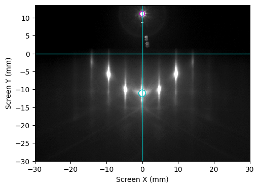
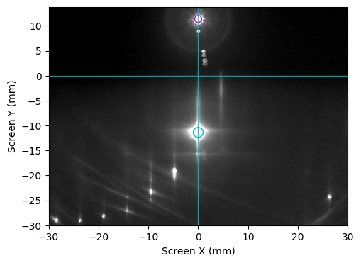
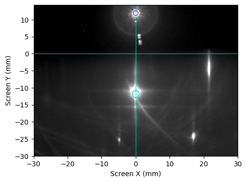
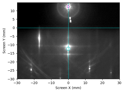
# Plot diagnostics
rheed.ri.plot_image(
show_center_lines=True,
show_specular_spot=True,
auto_levels=0.5
)
plt.title("")
plt.show()
Linear fits for interpolation across all images
slope, intercept = np.polyfit(selected_indices, center_x_samples, 1)
center_x_fit = all_indices * slope + intercept

slope, intercept = np.polyfit(selected_indices, center_y_samples, 1)
center_y_fit = all_indices * slope + intercept

slope, intercept = np.polyfit(selected_indices, incident_angle_samples, 1)
incident_angle_fit = all_indices * slope + intercept

arheed.ri.set_center_manual(center_x=center_x_fit, center_y=center_y_fit)

alpha_coords = np.linspace(0.0, 29.6, n_images)
beta_coords = incident_angle_fit

arheed = arheed.assign_coords(
    alpha=("frame", alpha_coords),
    beta=("frame", beta_coords),
)

# Set screen ROI
arheed.ri.screen_roi_width = 30
arheed.ri.screen_roi_height = 40

# Optionally use high pass filter (could be applied to the whole stack)
arheed = high_pass_filter(arheed, sigma=2.0, threshold=0.7)
Prepare a Lattice Object for the Expected Reconstruction
To verify the alignment, we create a lattice object representing the expected (√3 × √3) R30° reconstruction.
This lattice will later be used by the Ewald object for spot calculation and overlay.
from xrheed.kinematics import Lattice

# Si(111)-(1x1)
si_111_1x1 = Lattice.from_surface_hex(a=3.84, label="(1x1)")

# Si(111)-(r3xr3)R30
si_111_r3 = Lattice.from_surface_hex(a=3.84 * np.sqrt(3), label="(√3 x √3)")
si_111_r3.rotate(30)
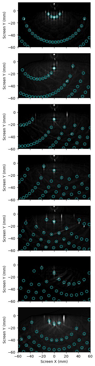
Generate Ewald Object and Overlay Expected Spot Positions
We generate an Ewald objects and use it to overlay the expected spot positions on each image.
This allows for visual verification of the alignment and consistency across the dataset.
Note: The
Ewaldobject could take a stack of images. In such case astack_indexproperty could be used to select a particular image from a stack.
from xrheed.kinematics import Ewald

arheed.ri.screen_roi_width = 60
arheed.ri.screen_roi_height = 60

ew = Ewald(si_111_r3, arheed)

fig, axs = plt.subplots(n_images, 1, sharex=True, figsize=(4.0, 14))

for idx in range(n_images):
    ax = axs[idx]
    # Select the image from the stack
    ew.stack_index = idx

    ew.plot(
        ax=ax, show_image=True,
        vmin=3, vmax=35,
        marker="o", facecolor="none", edgecolor="c", s=50,
    )
    ax.set_title("")
    if idx < n_images - 1:
        ax.set_xlabel("")

plt.tight_layout()
plt.show()
Transform Image Stack to kx–ky Space
If the alignment appears satisfactory, we proceed by transforming the whole image stack into the kx–ky space.
This step uses the arguments rotate=True and point_symmetry=True.
The
rotate=Trueoption applies a rotation around the image center by the azimuthal angle α.The
point_symmetry=Trueoption adds a mirrored image rotated by 180°, which is valid for most crystallographic structures.
from xrheed.conversion import transform_stack_to_kxky

kxky_stack = transform_stack_to_kxky(arheed, point_symmetry=True, rotate=True)
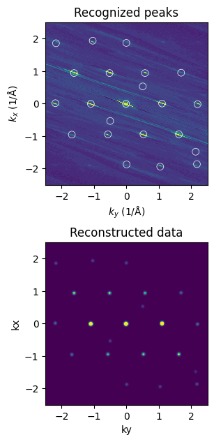
Find diffraction peaks in transformed data
RHEED diffraction spots often exhibit elongated shapes and additional inelastic scattering features.
After transforming a stack of images into reciprocal space (kx–ky), these effects may become further distorted or smeared.
The function filter_kspace_peaks localized in analysis module can be used to identify significant diffraction peaks and reconstruct the data using only the peak positions and their amplitudes. The reconstructed image replaces the experimental spot shapes with idealized Gaussian peaks, which is especially useful for averaging and comparing multiple transformed images.
Although the function can be applied directly to an entire stack, it is recommended to first tune the filtering parameters on a selected region or a single transformed image.
from xrheed.analysis import filter_kspace_peaks, plot_detected_peaks
Test filter on selected image
# selected frame
sel_idx = 4

# filter parameters
sigma_smooth = 0.13
min_peak_distance = 0.1
peak_percentile = 70
peak_width = 0.03

filtered, peaks = filter_kspace_peaks(
    kxky_stack[sel_idx],
    sigma_smooth=sigma_smooth,
    min_peak_distance=min_peak_distance,
    peak_percentile=peak_percentile,
    peak_width=peak_width,
    return_peaks=True,
)

fig, axs = plt.subplots(2, 1, figsize=(3.0, 7.5))
ax = axs[0]
plot_detected_peaks(
    kxky_stack[sel_idx], peaks, ax=ax, vmin=0, vmax=25, edgecolors="w", s=50
)

ax.set_title("Recognized peaks")
ax.set_xlim(-2.5, 2.5)
ax.set_ylim(-2.5, 2.5)

ax = axs[1]
filtered.plot(ax=ax, add_colorbar=False, vmin=0, vmax=25)

ax.set_title("Reconstructed data")
ax.set_xlim(-2.5, 2.5)
ax.set_ylim(-2.5, 2.5)
ax.set_aspect(1.0)

plt.show()
Finally, apply filter to the whole stack.
kxky_stack_filtered = filter_kspace_peaks(
    kxky_stack,
    sigma_smooth=sigma_smooth,
    min_peak_distance=min_peak_distance,
    peak_percentile=peak_percentile,
    peak_width=peak_width,
)
Compute the Mean Along the Azimuthal Dimension
Calculate the mean of the dataset for all frames.
This operation reduces the data to a single representative image, averaging over all angular orientations.
kxky_stack_mean = kxky_stack_filtered.mean(dim="frame")
Prepare the Final Plot
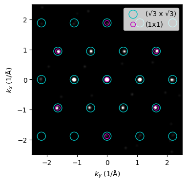
Finally, we generate an image that displays the mean intensity across all frames, along with overlays of the (1×1) and (√3 × √3) R30° reciprocal lattices for comparison.
As observed, the diffraction spots are elongated along several directions.
This elongation is a characteristic feature of RHEED, resulting from the finite domain size, which affects the shape of the diffraction spots.
Nonetheless, in this representation, it is straightforward to identify specific surface reconstructions, their symmetries, and mutual orientations.
fig, ax = plt.subplots(1, 1, figsize=(4, 4))

kxky_stack_mean.plot(ax=ax, cmap="gray", add_colorbar=False, vmin=0, vmax=10)

si_111_r3.plot_reciprocal(ax=ax, facecolor="none", edgecolor="c", s=150)
si_111_1x1.plot_reciprocal(ax=ax, facecolor="none", edgecolor="m", s=50)

ax.set_aspect(1)
ax.set_facecolor("black")
ax.set_xlim(-2.5, 2.5)
ax.set_ylim(-2.5, 2.5)
ax.legend(loc="upper right")
ax.set_title("")

plt.show()