Transforming into k-space

This notebook demonstrates how to use the Ewald module to convert a RHEED image coordinates into the \(k_x\)–\(k_y\) space.

import matplotlib.pyplot as plt
import numpy as np
from pathlib import Path

import xrheed

🎉 xrheed v2.1.0 loaded!

Prepare the Data

While not strictly required, it is recommended to first prepare the RHEED data by properly aligning the image. You should also verify the spot positions by comparing them with the points calculated using the Ewald module, as illustrated below.

image_dir = Path("example_data")
image_path = image_dir / "Si_111_r3Ag_112_thC.raw"

rheed_image = xrheed.load_data(image_path, plugin="dsnp_arpes_raw")

# Rotate the image
rheed_image.ri.rotate(-0.5)

# Manually pre-adjust the image center
center_x = -5.8
center_y = 0.2

rheed_image.ri.set_center_manual(center_x=center_x, center_y=center_y)

# Set the screen scale
#rheed_image.ri.screen_scale = 9.05

# Setup the screen roi
rheed_image.ri.screen_roi_width = 50
rheed_image.ri.screen_roi_height = 40

rheed_image.ri.set_center_auto(update_incident_angle=True)
# Prepare the plot
fig, ax = plt.subplots()

# Use automatic levels adjustment
rheed_image.ri.plot_image(
    ax=ax, auto_levels=0.2, show_center_lines=True, show_specular_spot=True
)

# add horizontal line to check the rotation alignment
ax.axhline(-58, color="m", linewidth=1.0)

plt.show()

Use a High-Pass Filter

Applying a high-pass filter before the transformation is highly recommended, as it enhances the visibility of diffraction features by suppressing background intensity.

from xrheed.preparation.filters import high_pass_filter

# Setup the screen roi
rheed_image.ri.screen_roi_width = 60
rheed_image.ri.screen_roi_height = 90

sigma = 1.5
threshold = 0.8

hp_rheed_image = high_pass_filter(rheed_image, sigma=sigma, threshold=threshold)
hp_rheed_image.ri.plot_image(auto_levels=0.3)

plt.show()

rheed_image = hp_rheed_image

Prepare the 2D Lattice

In this step, we define two lattices:

• Si(111)-(1×1) surface structure,

• \((\sqrt{3} \times \sqrt{3})\text{R}30^\circ\) reconstruction;

which is induced by the presence of 1 monolayer (ML) of Ag deposited at 500 °C.

from xrheed.kinematics import Lattice

si_111_1x1 = Lattice.from_surface_hex(a=3.84, label="(1x1)")
si_111_1x1.rotate(0.0)

si_111_r3 = Lattice.from_surface_hex(a=3.84 * np.sqrt(3), label="r3-Ag")
si_111_r3.rotate(30.0)

fig, ax = plt.subplots()

si_111_r3.plot_reciprocal(ax=ax, space_size=2.5, s=10, color="b")
si_111_1x1.plot_reciprocal(ax=ax, space_size=2.5, s=20, color="r")

ax.legend(loc="upper right")
plt.show()

Ewald Object

Create an instance of the Ewald class using the generated Si(111)-(1×1) lattice and the RHEED image.

If the RHEED image is properly aligned and scaled—and the lattice matches the actual crystal structure—there should be a good visual match between the calculated and observed diffraction spots, as shown below.

If the match is poor, return to the previous cells and adjust parameters such as shift_x, shift_y, screen_scale and beta directly on the image object. Then re-run all cells to recreate the Ewald object with the updated settings.

For convenience, these parameters can initially be adjusted only within the Ewald object. However, for accurate results, the RHEED image itself must ultimately be properly aligned.

from xrheed.kinematics import Ewald

ew_si_111_1x1 = Ewald(si_111_1x1, rheed_image)

fig, ax = plt.subplots()

# for testing only, finally apply those on the image before creating Ewald object
#ew_si_111_1x1.beta = 2.5
#ew_si_111_1x1.shift_x = 0.2
#ew_si_111_1x1.shift_y = -0.2
#ew_si_111_1x1.screen_scale = 9.05
#ew_si_111_1x1.ewald_azimuthal_rotation = 0.02

ew_si_111_1x1.plot(
    ax=ax,
    show_image=True,
    auto_levels=0.5,
    marker="o",
    facecolors="none",
    edgecolors="magenta",
    s=50,
)
plt.show()

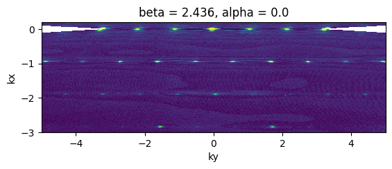
Final Transformation

The image can be transformed using the transform_image_to_kxky function.

Please note that the resulting image is no longer a RHEED image, and ri-related accessories are no longer available. Nonetheless, all attributes are copied from the original RHEED image for consistency.

from xrheed.conversion import transform_image_to_kxky

trans_image = transform_image_to_kxky(rheed_image, rotate=True, point_symmetry=True)

fig, ax = plt.subplots()

trans_image.plot(ax=ax, vmin=5, vmax=25, add_colorbar=False)

ax.set_xlim(-5, 5)
ax.set_ylim(-3, 0.2)
ax.set_aspect(1.0)
plt.show()

Final Plot with the Reciprocal Lattice

Finally, we can prepare a refined plot that displays both lattices overlaid in reciprocal space.

fig, ax = plt.subplots(figsize=(6, 6))

trans_image.plot(ax=ax, vmin=5, vmax=25, add_colorbar=False, cmap="gray")

si_111_r3.plot_reciprocal(ax=ax, facecolors="none", edgecolors="magenta", s=100)
si_111_1x1.plot_reciprocal(ax=ax, facecolors="none", edgecolors="cyan", s=150)

ax.set_xlim(-3.0, 3.0)
ax.set_ylim(-3.0, 3.0)
ax.set_aspect(1.0)
ax.set_facecolor("black")

ax.legend(loc="upper right")
plt.show()