Diffraction Profiles

This notebook demonstrates how to use xRHEED to extract a diffraction profile from a RHEED image.

As shown in the Getting Started notebook, the first step is to load the xrheed library and then import the RHEED image.

import matplotlib.pyplot as plt
import numpy as np
from pathlib import Path

import xrheed

🎉 xrheed v2.1.0 loaded!

image_dir = Path("example_data")
image_path = image_dir / "Si_111_7x7_112_phi_00.raw"

rheed_image = xrheed.load_data(image_path, plugin="dsnp_arpes_raw")
print(rheed_image.ri)

<RHEEDAccessor>
  File name: Si_111_7x7_112_phi_00.raw
  File creation time: 2026-04-24, 07:53:57
  Image shape: (1038, 1388)
  Screen scale: 9.3112 px/mm
  Screen sample distance: 309.2 mm
  Incident (beta) angle: 2.00 deg
  Azimuthal (alpha) angle: 0.00 deg
  Beam Energy: 19400.0 eV

Data Preparation

Before analyzing the RHEED image, it should be properly aligned. This may involve applying a rotation if necessary, and shifting the image horizontally and vertically to position the center accurately.

# Create a copy of the original RHEED image
aligned_image = rheed_image.copy()

# Apply rotation to correct image alignment
aligned_image.ri.rotate(-0.4)

# Replace the original image with the rotated version for further analysis
rheed_image = aligned_image

# Apply screen scaling correction if necessary
# Adjust based on exact calibration (here it should be 1.001857)
scaling_correction_factor = 1.0
rheed_image.ri.screen_scale *= scaling_correction_factor

# Set screen ROI
rheed_image.ri.screen_roi_width = 60
rheed_image.ri.screen_roi_height = 70

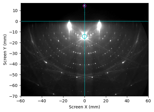
# Automatically determine and apply the image center after rotation
rheed_image.ri.set_center_auto(update_incident_angle=True)

# Use automatic levels adjustment
rheed_image.ri.plot_image(
    auto_levels=1.0, show_center_lines=True, show_specular_spot=True
)

plt.show()

Profile Extraction

Since the RHEED image is stored as a DataArray, a diffraction profile can be easily extracted using the built-in sel method, as shown below.

However, it is recommended to use the built-in accessor for profile extraction, which will be demonstrated later.

x_range = (-20, 20)  # in mm
y_range = (-10, 0)   # in mm

profile = rheed_image.sel(sx=slice(*x_range), sy=slice(*y_range)).mean("sy")

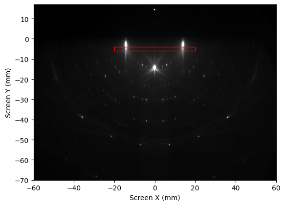
Profile Extraction Using the get_profile Method

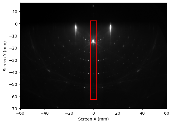
The get_profile method, available through the ri accessor, can also be used to extract a diffraction profile by specifying the center point, width, and height of the region.

Additionally, this function can plot the RHEED image with the profile region highlighted by setting plot_origin=True.

profile = rheed_image.ri.get_profile(
    center=(0, -5), width=40, height=2, show_origin=True
)

The rp accessor provides basic information about the extracted profile, making it easier to inspect and interpret the data.

profile.rp

<RHEEDProfileAccessor>
  Center: sx, sy [mm]: (0, -5) 
  Width: 40 mm
  Height: 2 mm
  Reduce over: sy
  Reduce method: mean

A RHEED profile retains the attributes of its parent image, ensuring consistency in metadata and coordinate references.

profile.ri

<RHEEDAccessor>
  File name: Si_111_7x7_112_phi_00.raw
  File creation time: 2026-04-24, 07:53:57
  Image shape: (373,)
  Screen scale: 9.3112 px/mm
  Screen sample distance: 309.2 mm
  Incident (beta) angle: 2.65 deg
  Azimuthal (alpha) angle: 0.00 deg
  Beam Energy: 19400.0 eV

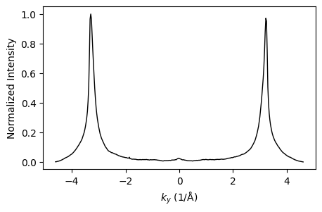
Plotting the Profile

The plot_profile function, accessible via the ri accessor, is used to visualize the extracted profile. It supports additional parameters such as normalize and transform_to_k.

When transform_to_k=True, the profile is plotted using a temporary scattering coordinate, \(k_y\), which provides a momentum-resolved representation of the diffraction data.

Note: In the coordinate system used by the xRHEED project, the screen’s horizontal axis (x-coordinate) is parallel to \(k_y\) in momentum space. For further details, refer to the Geometry section of the documentation.

profile.rp.plot_profile(
    transform_to_k=True, normalize=True, color="black", linewidth=1.0
)

plt.show()

Converting the Profile to \(k_y\)

The profile can be permanently converted to momentum space coordinates using the dedicated ri.convert_to_k method.

profile_k = profile.rp.convert_to_k()

Profile Fitting

The diffraction profile can be fitted using the lmfit library, as demonstrated in the example below.

from lmfit.models import LorentzianModel, QuadraticModel

# Extract data from profile
x = profile_k.coords["ky"].values
y = profile_k.values

# Preprocess: remove background offset and normalize
y = y - np.min(y)
y = y / np.max(y)

# Define individual models
l1 = LorentzianModel(prefix="l1_")
l2 = LorentzianModel(prefix="l2_")
bkg = QuadraticModel(prefix="bkg_")

# Combine into a composite model
model = l1 + l2 + bkg

# Initialize parameters with reasonable guesses
params = model.make_params()
params["l1_center"].set(value=-3.0)
params["l1_amplitude"].set(value=1.0)
params["l1_sigma"].set(value=0.1)

params["l2_center"].set(value=3.0)
params["l2_amplitude"].set(value=1.0)
params["l2_sigma"].set(value=0.1)

params["bkg_a"].set(value=-1.0)
params["bkg_b"].set(value=0.0)
params["bkg_c"].set(value=0.0)

# Perform the fit
result = model.fit(y, params, x=x)

# Plot the fit result
result.plot_fit(title="RHEED Profile Fit")
plt.show()

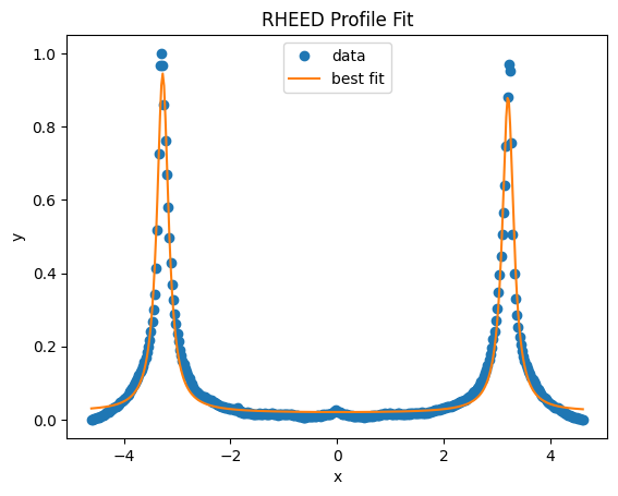
# Calculate half the distance between the two fitted peaks
half_peak_distance = 0.5 * (
    result.params["l2_center"].value - result.params["l1_center"].value
)

print(f"Half peak distance from the specular reflection: {half_peak_distance:.2f} 1/Å")

# Expected peak separation for Si(111)-(1×1) along the [110] direction
expected_distance = 4 * np.pi / 3.84  # 1/A
print(f"Expected peak separation: {expected_distance:.2f} 1/Å")

Half peak distance from the specular reflection: 3.24 1/Å
Expected peak separation: 3.27 1/Å

Fine Adjustment of the Screen Scale

The measured distance between the two diffraction peaks can be used to refine the screen scale. If the measured peak separation differs from the expected value, the scale factor may require adjustment to ensure accurate momentum calibration.

scaling_correction = half_peak_distance / expected_distance

print(f"Calculated correction of the screen scale: {scaling_correction:.6f}")

rheed_image.ri.screen_scale *= scaling_correction

Calculated correction of the screen scale: 0.989816

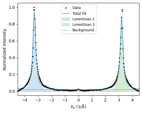
Preparing a Final Plot

Generate a final plot with a polished appearance to clearly present the fitted RHEED profile and highlight key features.

# Evaluate components
comps = result.eval_components(x=x)

# Create figure
fig, ax = plt.subplots(figsize=(5, 4), tight_layout=True)

# Plot data and total fit
ax.plot(x, y, "ko", markersize=2, label="Data")  # black dots for data
ax.plot(
    x, result.best_fit, color="tab:blue", linestyle="-", linewidth=1, label="Total Fit"
)

# Plot Lorentzian components as shaded areas
for i, color in zip(range(1, 3), ["tab:blue", "tab:green", "tab:purple"]):
    comp = comps[f"l{i}_"]
    ax.fill_between(x, comp, color=color, alpha=0.2, label=f"Lorentzian {i}")

# Plot background as a dashed line
ax.plot(
    x, comps["bkg_"], color="gray", linestyle="--", linewidth=1.0, label="Background"
)

# Labels and styling
ax.set_xlabel("$k_y$ (1/Å)", fontsize=10)
ax.set_ylabel("Normalized Intensity", fontsize=10)

# Legend outside the plot area
ax.legend(fontsize=9)
ax.set_xlim(-4.5, 4.5)

plt.show()

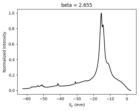
Vertical Profiles

By default, profiles are averaged over the sy (vertical) direction. This is because, in the defined geometry, sx corresponds to the sample’s ky direction, which is perpendicular to the electron beam.

However, profiles can also be computed by averaging or summing over sx if the reduce_over argument is provided, as shown below.

vertical_profile = rheed_image.ri.get_profile(
    center=(0, -30),
    width=5,
    height=65,
    reduce_over="sx",
    method="mean",
    show_origin=True,
)
plt.show()

vertical_profile.rp

<RHEEDProfileAccessor>
  Center: sx, sy [mm]: (0, -30) 
  Width: 5 mm
  Height: 65 mm
  Reduce over: sx
  Reduce method: mean

fig, ax = plt.subplots(figsize=(5, 4), tight_layout=True)

vertical_profile.rp.plot_profile(ax=ax, color="k")
plt.show()